
Solution
1
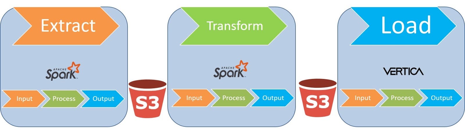
Extract
Let’s assume that we want to extract data from RDBMS (in our example, we’ll use MS SQL Server). Given that your table structure can be different, the most effective way to upload data is to use an integer key with uniform data distribution.
This works especially well when there is a clustered index on the key column or nonclustered index which includes all the fields you need. Assuming that we need to read all data (not a part, a half, or a row).
Our goal is to read the entire table in the shortest possible time. We’ll divide the table into parts so that we can process several data streams simultaneously.
The use of integer key
To apply the integer key, take the minimum and maximum values so that you get a range of all presented values in this table.
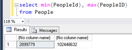
Spark technology provides a basic functionality where you specify these limit values, the table and the column where you need to partition your data. Spark will do the rest for you.
sQLContext.read.jdbc(url=url,
table=”People”,
columnName=”PeopleId”,
lowerBound=2899779,
upperBound=102448632,
numPartitions=200,
connectionProperties=connectionProperties
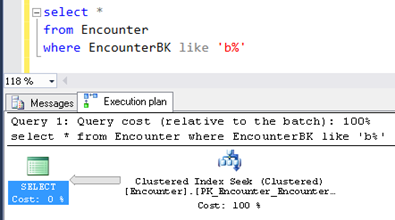
)On the screen, you can see an approximate request launched by Spark.
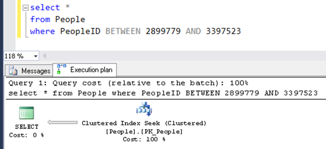
It’s a request to one of the partitions where it independently calculates limit values to this part of the table. The effectiveness of the operation depends on the table itself. The execution plan shows a “Clustered Index Seek”, which is a fairly useful feature.
A “Clustered Index Scan” should show that the operation is ineffective for this particular case. A scan index means that each of 200 partitions will scan the entire table to find its own one.
Thus, the integer key with a clustered index is a perfect solution as it ensures a sequential efficient read. Even with a nonclustered index, it still works. Just make sure that all table fields are included in the index since with incomplete information, a nonclustered index will refer to the clustered one to take data from it. And finally, you’ll get inconsequential ineffective read with an increased disk load.
The main advantage is that you don’t need to scan the whole table to divide it into the parts and understand what values it contains. All you need is to determine min and max values using an integer key.
The use of varchar key
You can also face a situation when your key is represented by a text field. In comparison to the integer key, when you add some amount and get another limit value, the varchar key with a text value becomes a real puzzle.
How to split the table into N approximately equal parts? You can dynamically number a table records to have integer key, but, this requires scanning of the entire table.
A snag is that we don’t want to waste five minutes to scan it and then spend 10 more minutes to read it piece by piece. We want to start reading it immediately.
Here we can split a table by first N characters of the text key and apply LIKE operator to achieve “Index Seek” when reading a single part. Unfortunately, Spark does not provide such functionality, so we need to implement it.
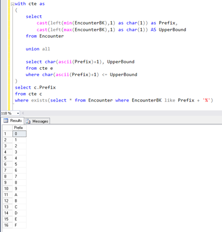
Here we deal with a request made based on the min and max values, and their first symbols. To generate all sorts of combinations, you can go through the table and check if those values are there. This will be quite effective as you can use search by index.
What if you use files instead of the database as a source of data?
Rule 1. Use a scalable storage system, such as HDFS or S3.
Rule 2. Use multiple files as you can process them through multiple streams. Even if you have a single file, try to divide it so several processes will read them at the same time.
Rule 3. Use splittable file formats and compression. Example:
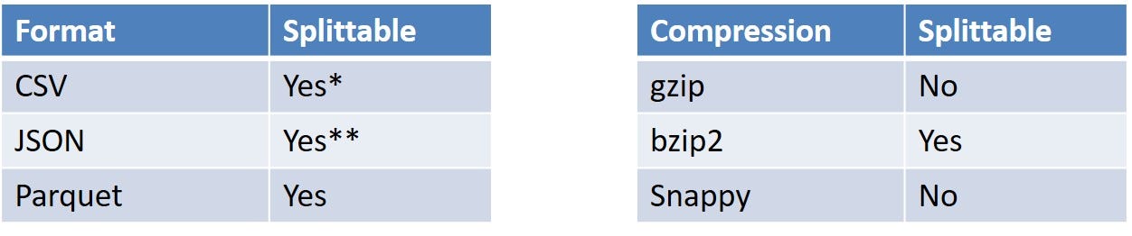
* CSV is splittable when it is a raw, uncompressed file or using a splittable compression format such as BZIP2
** JSON has the same conditions about splittability when compressed as CSV with one extra difference. When “wholeFile” option is set to true (re: SPARK-18352), JSON is NOT splittable.
How to effectively store data?
Rule 1. Use scalable storage: HDFS, S3, etc.
- Hint: To avoid the full data copy from Spark on S3, add the Spark property mapreduce.fileoutputcommitter.algorithm.version = 2. Thus, your data will be stored only once.
- If you work on Amazon, use EMR 5.20.0 or later.
Rule 2. Store multiple files to speed uploading.
Results
- EMR 5.20.0 with 10 instances (c4.4xlarge)
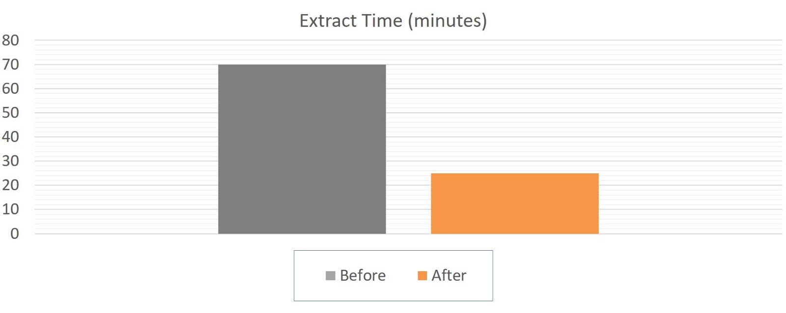
- Input: 3 Databases (MS SQL), ~ 400 GB (raw data)
- Output: Parquet (Snappy), ~ 100 GB
We sped up the Extract time by almost three times. See the graph.
2
Transform
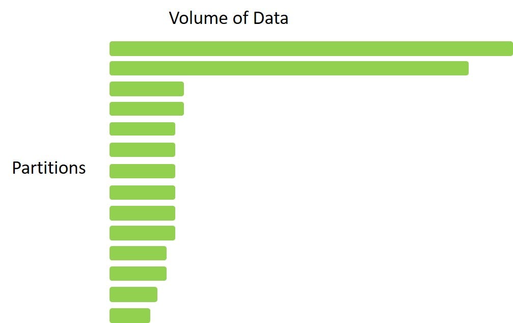
Data Skew
A distinctive feature of all distributed processing systems, including Spark, is irregular data distribution. If you read a file or information in a database, and you have a cluster with 10 machines, then, 90 percent of all data can be distributed within only one machine while 10 percent will get in other nine machines.
Surely, such a distribution isn’t effective as a system will process small partitions much quicker than the remaining huge ones, which can last for hours. Pay special attention to the choice of a key that you’re going to use to distribute data (we still recommend the integer key with excellent distribution!).
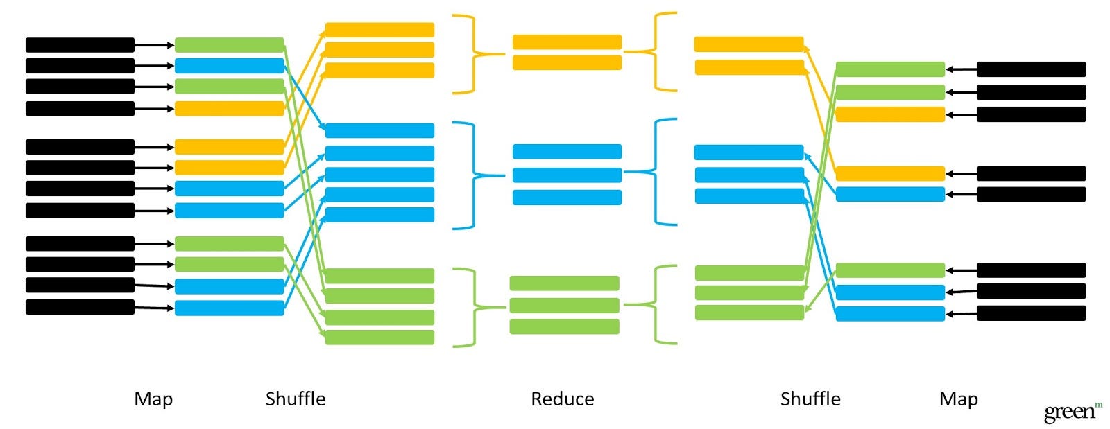
Join
The next pivotal feature of data processing in distributed systems comes into action when you try to join two tables. This can be one of two typical ways:
1) Shuffle join. Two tables are large and a machine doesn’t have enough memory to store any of them.
A solution can be to distribute the tables throughout the whole cluster and join them somehow. Here’s how it looks on practice: you don’t have access to data so that you make a request and ask to join.
Your data are divided into groups and distributed throughout the cluster in a way that a single key appears on the same node. That’s how joining occurs. This complex operation is called shuffle, and if you have an abundance of data, most of all the processing time will be spent on shuffles.
* SELECT * FROM Encounters e JOIN Providers p ON e.ProviderId = p.ProviderId
2) Broadcast join. One table is large and you can’t store it in one node, and the second one is small. Such a kind of join will be fast and effective. With no need for doing shuffle operations, you just assemble the small table in one place and copy it to all nodes. In this way, you shouldn’t distribute the large table across the key.
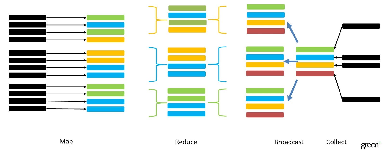
* SELECT * FROM Encounters e JOIN Providers p ON e.ProviderId = p.ProviderId
How to reduce shuffles?
- Use data partitioning, bucketing
- Broadcast small tables when joining them to the big table:
spark.sql.autoBroadcastJoinThreshold= 10485760 (10 MB – default)
- Use COUNT (key) instead of COUNT (DISTINCT key) if possible
- Drop unused data
- Filter/reduce before join
- Cache datasets used multiple times
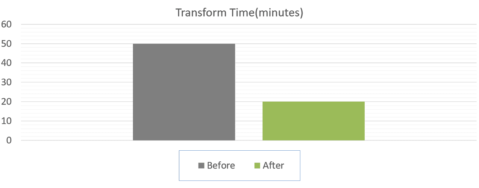
Results
- EMR 5.20.0 with 10 instances (c4.8xlarge)
- Input: Parquet(Snappy), 50GB
- Output: ORC(ZLib), 19GB
We accelerated the Transform time by more than two times. See the graph.
3
Load
The last stage in our data pipeline processing is load. We don’t use any special load processes and programs. Instead, we make a request with listed files (you can separate them by commas or just specify a mask). Then, Vertica on its own goes to S3, takes the list of files and distributes them between nodes.
Take into account that the load performance and scalability depends on the number of nodes in the cluster, number of files, file formats and destination table structure.
COPY dm1.FactTable
              (
              Column1,
              Column2,
              DateColumnTZ FILLER TIMESTAMPTZ,
              DateColumn AS DateColumnTZ AT TIME ZONE ‘UTC’,
              Column4,
              …
              )
              FROM ‘s3://bucket/prod/datamarts/dm1/FactTable/snapshots/snapshotid=20190418/part-*.orc’
              ORC
              DIRECT
            ABORT ON ERROR;
Results
- Input: ORC(ZLib), 19GB
- Output: Vertica DB (7 Node)
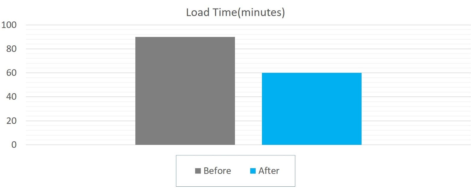
Finally, we launched an ETL process that is able to scale.
Technology used
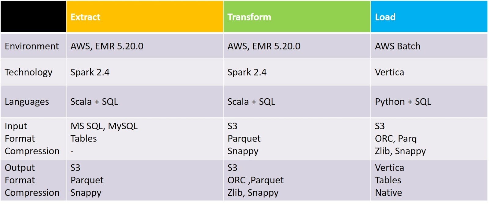
Fantastic Four
In summary, we want to conclude with four critical rules to follow when developing a product.
First and foremost, always remember its scalability. Functionality that works today may fail tomorrow under new circumstances.
Secondly, multiply all data you’re going to work by two, three or five times. Consider tomorrow’s data volume.
The third rule is that you should build with failure in mind.
Finally, the last rule is to consider risk management. Understand the potential risks of your app and be ready to respond.